Score-Based Diffusion Models
Theory from single noise perturbation to SDE formulation and application to image generation
The goal of this project is to derive, from scratch, a score-based generative model based on a stochastic differential equation (SDE), inspired by the following paper:
Song et al., “Score-Based Generative Modeling through Stochastic Differential Equations” (2021)
Generative Modeling
Let $\mathcal{D} = {x_1, \dots, x_n}$ be a dataset of $i.i.d.$ samples from an unknown distribution $p(x)$ , with $x \in \mathbb{R}^D$. The goal of generative modeling is to learn a model $p_\theta(x)$ that approximates $p(x)$, enabling the generation of new, realistic samples. When $p_\theta(x)$ is parameterized by a neural network, we refer to it as a deep generative model.
As noted by Yang Song, generative models can be broadly categorized based on how they represent probability distributions:
How to represent a probability distribution
One way to represent a probability distribution is to directly model the probability density function (p.d.f.). For example, we can use a real-valued function $f_\theta(\mathbf{x})$, parameterized by a learnable parameter $\theta$, to define:
\[p_\theta(x) = \frac{e^{-f_\theta(\mathbf{x})}}{Z(\theta)}\]Here, $f_\theta(\mathbf{x})$ is often referred to as the energy function, $p_\theta(x)$ as an energy-based model, and $Z(\theta)$ is a normalizing constant dependent on $\theta$, such that:
\[\int_{\mathbb{R}^d} p_\theta(x) \, dx = 1.\]These models are typically trained using (exact or approximate) maximum likelihood estimation (MLE):
\[\boxed{\theta^*_{\text{MLE}} = \arg\max_\theta \sum_{i=1}^n \log p_\theta(x_i)}\]However, computing $p_\theta(x)$ requires evaluating the normalizing constant $Z(\theta)$ — a typically intractable quantity for any general $f_\theta(\mathbf{x})$. For instance, image data implies $x \in \mathbb{R}^{3 \times H \times W}$, video data implies $x \in \mathbb{R}^{T \times 3 \times H \times W}$ and time series implies $x \in \mathbb{R}^{C \times T}$. Such data can easily reach hundreds of thousands of dimensions.
Overview of generative modeling
Thus, to make maximum likelihood training feasible, likelihood-based models must either restrict their model architectures (e.g. invertible networks in normalizing flow models) to make $Z(\theta)$ tractable, or approximate the normalizing constant (e.g., variational inference in variational autoencoders) which may be computationally expensive.
Another way to represent a probability distribution is by implicit generative models, where the distribution is implicitly represented by a model of its sampling process. The most prominent example is generative adversarial networks which learn to generate realistic samples by transforming Gaussian noise through a neural network, and are trained via a two-player minimax game between a generator and a discriminator. Unlike likelihood-based models, there is no tractable expression for the density $p_\theta(x)$, which makes likelihood-based training infeasible.
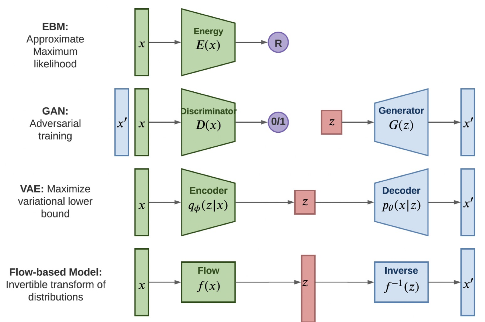
| EBM: | Learn an unnormalized distribution by assigning low energy to likely data; trained via approximate maximum likelihood. |
| GAN: | Generate realistic data through a minimax game between generator and discriminator; trained via adversarial optimization. |
| VAE: | Encode data into a latent space and decode it; trained by maximizing a variational lower bound. |
| Flow-based: | Use invertible mappings to transform between data and latent variables; trained via exact maximum likelihood. |
Score-based Generative Modeling
Likelihood-based models and implicit generative models, however, both have significant limitations. Likelihood-based models either require strong restrictions on the model architecture to ensure a tractable normalizing constant for likelihood computation, or must rely on surrogate objectives to approximate maximum likelihood training. Implicit generative models, on the other hand, often require adversarial training, which is notoriously unstable and can lead to mode collapse.
Score function
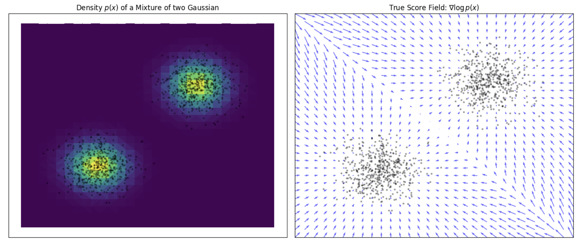
As shown by Hyvärinen (2005), another approach to generative modeling is to model the gradient of the log probability density function instead of the density function itself. This produces a quantity often known as the score function. By modeling the score function instead of the density function, we can sidestep the difficulty of intractable normalizing constants.
The score function of a distribution $p(\mathbf{x})$ is defined as
\[\nabla_{\mathbf{x}} \log p(\mathbf{x}),\]and a model for the score function is called a score-based model, which we denote as $s_\theta(\mathbf{x})$.
The score-based model is learned such that
\[\boxed{s_\theta(\mathbf{x}) \approx \nabla_{\mathbf{x}} \log p(\mathbf{x})}\]and can be parameterized without worrying about the normalizing constant $Z_\theta$.
Indeed, if we take the example of an energy-based model we obtain:
\[s_\theta(\mathbf{x}) \approx \nabla_{\mathbf{x}} \log p(\mathbf{x}) = \nabla_{\mathbf{x}} \log \frac{e^{-f_\theta(\mathbf{x})}}{Z_\theta} = \nabla_{\mathbf{x}} \log e^{-f_\theta(\mathbf{x})} - \underbrace{\nabla_{\mathbf{x}} \log Z_\theta}_{= 0} = - \nabla_{\mathbf{x}} f_\theta(\mathbf{x})\]Note that $s_\theta(\mathbf{x}) \in \mathbb{R}^D$ when $\mathbf{x} \in \mathbb{R}^D$.
This significantly expands the family of models that we can tractably use, since we don’t need any special architectures to make the normalizing constant tractable. The only constraint is that the model output must have the same dimension as the input.
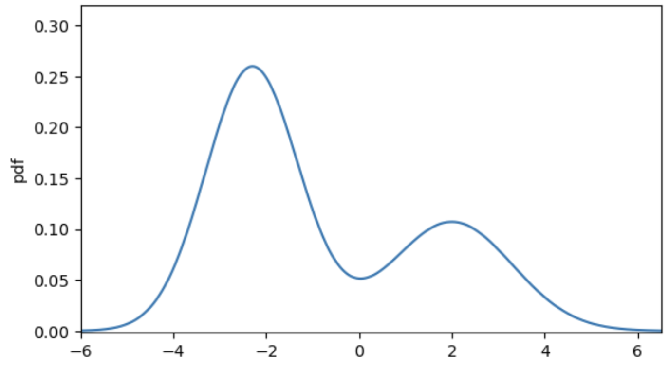
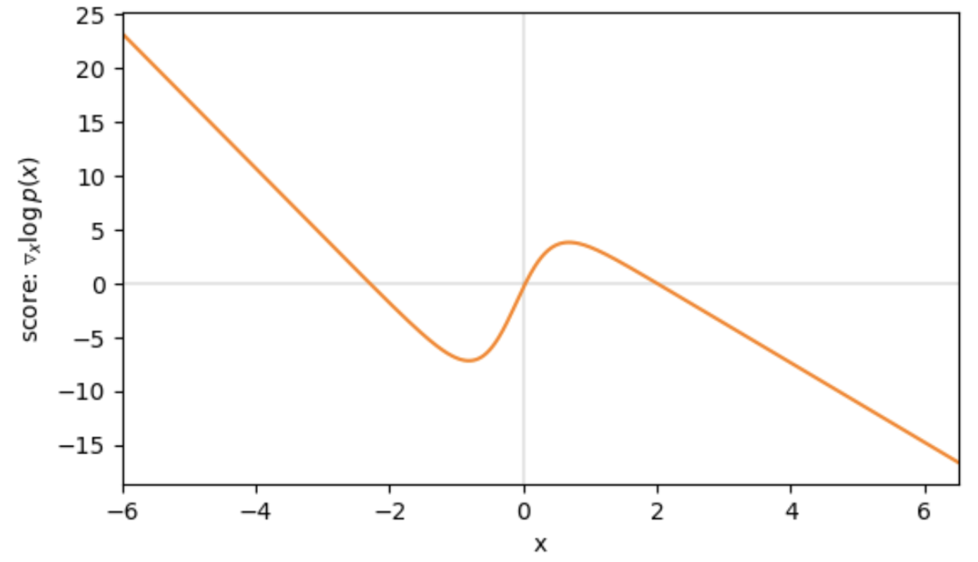
Let’s assume our true data distribution is a simple univariate Gaussian Mixture Model (GMM), as displayed in the following figure. The value of the corresponding score function at each position $x$, tells us the direction of higher density. For example, if we are at $x = -4$ we can see that the score is positive and thus, if we want to make $x$ slightly more likely under $p(x)$, we need to move to the right. Contrarily, if we evaluate the point $x = 4$, the negative score tells us that for a higher density region we need to move to the left.
Learning Scores via Score Matching
Instead of fitting a model to the data distribution, we can fit a model to the score function. The score function is a gradient; therefore, it returns an object of the same shape as its input $x$. Thus, similar to likelihood-based models, we can train score-based models by minimizing the Fisher divergence between the model and the data distributions.
Fisher divergence is typically between two distributions $p$ and $q$, defined as
\[\boxed{ fisher(p \mid q) = \mathbb{E}_{x\sim p} \left[ \left\| \nabla_{\mathbf{x}} \log p(\mathbf{x}) - \nabla_{\mathbf{x}} \log q(\mathbf{x}) \right\|^2 \right]}\]Here we slightly abuse the term as the name of a closely related expression for score-based models.
So the function we want to minimize to learn the score is defined as follows:
\[\boxed{ L_{\text{ESM}_{p}}(\theta) = \mathbb{E}_{x\sim p} \left[ \left\| \, s_\theta(\mathbf{x}) - \nabla_{\mathbf{x}} \log p(\mathbf{x}) \right\|^2 \right] = \int_{\mathbb{R}^D} \left\| s_\theta(\mathbf{x}) - \nabla_{\mathbf{x}} \log p(\mathbf{x}) \right\|^2 p(\mathbf{x}) \, d\mathbf{x}.}\]Following the terminology introduced by Vincent (2010), we will refer to this objective loss function as explicit score matching (ESM).
Finally, the minimizer $\theta^*$ of this function, which corresponds to the model’s optimal parameters, is defined by:
\[\theta^* = \arg\min_\theta L_{\text{ESM}}(\theta)\]Following the terminology introduced by Hyvärinen (2005), we will refer to $\theta^*$ as the score matching estimator.
Sampling with Langevin Dynamics
Once we have trained a score-based model $s_\theta(\mathbf{x}) \approx \nabla_{\mathbf{x}} \log p(\mathbf{x})$, we can use an iterative procedure called Langevin dynamics to draw samples from it. Langevin dynamics provides a procedure to sample from a distribution $p(\mathbf{x})$ using only its score function $\nabla_{\mathbf{x}} \log p(\mathbf{x}).$
The method is based on simulating the following stochastic differential equation (SDE):
\[\boxed{ d\mathbf{x}_t = \nabla_{\mathbf{x}} \log p(\mathbf{x}_t) \, dt + \sqrt{2} \, d\mathbf{w}_t}\]where $\mathbf{w}_t$ is standard Brownian motion.
This SDE defines a stochastic process whose stationary distribution is $p(\mathbf{x})$, under regularity conditions. We discretize this SDE using a step size $\Delta t$, initializes from an arbitrary prior distribution $\mathbf{x}_0 \sim \pi(\mathbf{x})$, and then iterates the following:
\[\boxed{ \mathbf{x}_{i+1} \leftarrow \mathbf{x}_i + \Delta t \nabla_{\mathbf{x}} \log p(\mathbf{x}) + \sqrt{2\Delta t} \, \mathbf{z}_i, \quad i = 0, 1, \cdots, K,}\]where $\mathbf{z}_i \sim \mathcal{N}(0, \mathbf{I})$. When $\Delta t \to 0$ and $K \to \infty$, $\mathbf{x}_K$ obtained from the procedure converges to a sample from $p(\mathbf{x})$ under some regularity conditions. In practice, the error is negligible when $\Delta t$ is sufficiently small and $K$ is sufficiently large.
The gradient term $\Delta t \nabla_{\mathbf{x}} \log p(\mathbf{x}_i)$ moves samples toward regions of high probability. The noise term $\sqrt{2\Delta t} \mathbf{z}_i$ ensures randomness and exploration, preventing the chain from collapsing to modes.
Proof.
Let $p_t(\mathbf{x})$ be the density at time $t$. It evolves according to the Fokker–Planck equation:
\[\boxed{\frac{\partial p_t(\mathbf{x})}{\partial t} = -\nabla_{\mathbf{x}} \cdot \left( p_t(\mathbf{x}) \nabla_{\mathbf{x}} \log p(\mathbf{x}) \right) + \nabla_{\mathbf{x}}^2 p_t(\mathbf{x}).}\]A stationary solution $\bar{p}(\mathbf{x})$ of the Fokker–Planck equation is a time-independent probability density that satisfies:
\[\frac{\partial \bar{p}(\mathbf{x})}{\partial t} = 0.\]Substituting into the Fokker–Planck equation yields the condition:
\[-\nabla_{\mathbf{x}} \cdot \left( \bar{p}(\mathbf{x}) \nabla_{\mathbf{x}} \log p(\mathbf{x}) \right) + \nabla_{\mathbf{x}}^2 \bar{p}(\mathbf{x}) = 0.\]Let us assume that $p(\mathbf{x})$ is a smooth, strictly positive density with support on $\mathbb{R}^d$, and define:
\[\bar{p}(\mathbf{x}) := p(\mathbf{x}).\]Then:
\[\begin{align*} -\nabla_{\mathbf{x}} \cdot \left( \bar{p}(\mathbf{x}) \nabla_{\mathbf{x}} \log p(\mathbf{x}) \right) + \nabla_{\mathbf{x}}^2 \bar{p}(\mathbf{x}) &= -\nabla_{\mathbf{x}} \cdot \left( p(\mathbf{x}) \nabla_{\mathbf{x}} \log p(\mathbf{x}) \right) + \nabla_{\mathbf{x}}^2 p(\mathbf{x}) \\ &= -\nabla_{\mathbf{x}} \cdot \left( \nabla_{\mathbf{x}} p(\mathbf{x}) \right) + \nabla_{\mathbf{x}}^2 p(\mathbf{x}) \\ &= -\nabla_{\mathbf{x}}^2 p(\mathbf{x}) + \nabla_{\mathbf{x}}^2 p(\mathbf{x}) \\ &= 0 \end{align*}\]Therefore, the stationary solution of this PDE is exactly $p(\mathbf{x})$:
\[\boxed{ \lim_{t \to \infty} p_t(\mathbf{x}) = p(\mathbf{x})}.\]Note that Langevin dynamics accesses $p(\mathbf{x})$ only through $\nabla_{\mathbf{x}} \log p(\mathbf{x})$. Since $s_\theta(\mathbf{x}) \approx \nabla_{\mathbf{x}} \log p(\mathbf{x})$, we can produce samples from our score-based model $s_\theta(\mathbf{x})$ by plugging it into the iterative procedure.
Limitations of explicit score matching
We’ve discussed how to train a score-based model with score matching, and then produce samples via Langevin dynamics. However, as showed by Song & Ermon (2020), this naive approach has had limited success in practice.
First, it requires us to have access to the true score of the data distribution, which we usually don’t have. And second, it fails to learn good estimates of the score in low density regions, where few data points are available for computing the score matching objective.
This is expected as score matching minimizes the Fisher divergence:
\[L_{\text{ESM}_{p}}(\theta) = \int_{\mathbb{R}^D} \left\| s_\theta(\mathbf{x}) - \nabla_{\mathbf{x}} \log p(\mathbf{x}) \right\|^2 p(\mathbf{x}) \, d\mathbf{x}.\]Since the $\ell_2$ differences between the true data score function and score-based model are weighted by $p(x)$, they are largely ignored in low density regions where $p(x)$ is small. This behavior can lead to subpar results.
When sampling with Langevin dynamics, our initial sample is highly likely in low density regions when data reside in a high dimensional space. Therefore, having an inaccurate score-based model will derail Langevin dynamics from the very beginning of the procedure, preventing it from generating high quality samples that are representative of the data.
Estimation of the true score
Hyvärinen (2005) proved the following remarkable property:
\[\boxed{ \underbrace{\mathbb{E}_{x\sim p} \left[ \left\| s_\theta(\mathbf{x}) - \nabla_{\mathbf{x}} \log p(\mathbf{x}) \right\|^2 \right]}_{L_{\text{ESM}_{p}}(\theta)} = \underbrace{\mathbb{E}_{x\sim p} \left[ \| s_\theta(\mathbf{x}) \|^2 + \sum_{i=1}^d \frac{\partial s_{\theta, i}(\mathbf{x})}{\partial x_i} \right] + C}_{L_{\text{ISM}_{p}}(\theta)} = \underbrace{\mathbb{E}_{x\sim p} \left[ \| s_\theta(\mathbf{x}) \|^2 + \mathrm{Tr}(\nabla_x s_{\theta}(\mathbf{x})) \right] + C}_{L_{\text{ISM}_{p}}(\theta)}}\]where $s_{\theta, i}(\mathbf{x})$ denotes the $i$-th component of $s_\theta(\mathbf{x})$, and $C$ is a constant that does not depend on $\theta$. This yields an implicit score matching objective $L_{\mathrm{ISM}{p}}$ that no longer requires having an explicit score target for $p(\mathbf{x})$, but is nevertheless equivalent to $L{\mathrm{ESM}_{p}}$.
Hyvärinen formally shows that, provided $p(\mathbf{x})$ and $s_\theta(\mathbf{x})$ satisfy some weak regularity conditions, we have:
\[L_{\text{ESM}_{p}} \;\sim\; L_{\text{ISM}_{p}}.\]Proof.
By developing the explicit score matching loss:
\[\begin{aligned} L_{\mathrm{ESM}_p}(\theta) &= \mathbb{E}_{\mathbf{x} \sim p} \left[ \| s_\theta(\mathbf{x}) \|^2 - 2 \, s_\theta(\mathbf{x})^\top \nabla_{\mathbf{x}} \log p(\mathbf{x}) + \| \nabla_{\mathbf{x}} \log p(\mathbf{x}) \|^2 \right] \\ &= \mathbb{E}_{\mathbf{x} \sim p} \left[ \| s_\theta(\mathbf{x}) \|^2 \right] - 2 \, \mathbb{E}_{\mathbf{x} \sim p} \left[ s_\theta(\mathbf{x})^\top \nabla_{\mathbf{x}} \log p(\mathbf{x}) \right] + \mathbb{E}_{\mathbf{x} \sim p} \left[ \| \nabla_{\mathbf{x}} \log p(\mathbf{x}) \|^2 \right]. \end{aligned}\]Let us denote the cross term:
\[\mathbb{E}_{\mathbf{x} \sim p} \left[ s_\theta(\mathbf{x})^\top \nabla_{\mathbf{x}} \log p(\mathbf{x}) \right] = \int_{\mathbb{R}^d} s_\theta(\mathbf{x})^\top \nabla_{\mathbf{x}} \log p(\mathbf{x}) \, p(\mathbf{x}) \, d\mathbf{x}.\]Using the identity $\nabla_{\mathbf{x}} \log p(\mathbf{x}) = \frac{\nabla_{\mathbf{x}} p(\mathbf{x})}{p(\mathbf{x})}$, this becomes:
\[\int_{\mathbb{R}^d} s_\theta(\mathbf{x})^\top \nabla_{\mathbf{x}} p(\mathbf{x}) \, d\mathbf{x}.\]We now apply integration by parts (assuming $p(\mathbf{x}) s_\theta(\mathbf{x})$ decay fast enough as $|\mathbf{x}| \to \infty$):
\[\int_{\mathbb{R}^d} s_{\theta,i}(\mathbf{x}) \frac{\partial p(\mathbf{x})}{\partial x_i} \, d\mathbf{x} = - \int_{\mathbb{R}^d} \frac{\partial s_{\theta,i}(\mathbf{x})}{\partial x_i} \, p(\mathbf{x}) \, d\mathbf{x},\]so summing over $i = 1, \dots, d$:
\[\int_{\mathbb{R}^d} s_\theta(\mathbf{x})^\top \nabla_{\mathbf{x}} p(\mathbf{x}) \, d\mathbf{x} = - \int_{\mathbb{R}^d} \mathrm{Tr}(\nabla_{\mathbf{x}} s_\theta(\mathbf{x})) \, p(\mathbf{x}) \, d\mathbf{x} = - \mathbb{E}_{\mathbf{x} \sim p} \left[ \mathrm{Tr}(\nabla_{\mathbf{x}} s_\theta(\mathbf{x})) \right].\]Substituting back into $L_{\mathrm{ESM}_p}$, we get:
\[L_{\mathrm{ESM}_p}(\theta) = \mathbb{E}_{\mathbf{x} \sim p} \left[ \| s_\theta(\mathbf{x}) \|^2 \right] + 2 \, \mathbb{E}_{\mathbf{x} \sim p} \left[ \mathrm{Tr}(\nabla_{\mathbf{x}} s_\theta(\mathbf{x})) \right] + C,\]where
\[C = \mathbb{E}_{\mathbf{x} \sim p} \left[ \| \nabla_{\mathbf{x}} \log p(\mathbf{x}) \|^2 \right]\]is a constant independent of $\theta$.
Thus, we conclude:
\[L_{\mathrm{ISM}_p}(\theta) := \mathbb{E}_{\mathbf{x} \sim p} \left[ \| s_\theta(\mathbf{x}) \|^2 + \mathrm{Tr}(\nabla_{\mathbf{x}} s_\theta(\mathbf{x})) \right],\]and:
\[L_{\mathrm{ESM}_p}(\theta) = L_{\mathrm{ISM}_p}(\theta) + C.\]Since we only have samples $D_n$ from $p(\mathbf{x})$, Hyvärinen proposes to optimize the finite-sample version of $L_{\mathrm{ISM}{p}}$, which we will write $L{\mathrm{ISM}_{p_n}}$.
\[L_{\mathrm{ISM}_{p_n}}(\theta) = \mathbb{E}_{\mathbf{x} \sim p_n} \left[ \| s_\theta(\mathbf{x}) \|^2 + \sum_{i=1}^d \frac{\partial s_{\theta, i}(\mathbf{x})}{\partial x_i} \right] = \frac{1}{n} \sum_{t=1}^n \left( \| s_\theta(\mathbf{x}) \|^2 + \sum_{i=1}^d \frac{\partial s_{\theta, i}(\mathbf{x})}{\partial x_i} \right).\]$L_{\mathrm{ISM}{p_n}}$ is asymptotically equivalent to $L{\mathrm{ISM}{p}}$ when $n \to \infty$, and hence asymptotically equivalent to objective $L{\mathrm{ESM}_p}$. This can be summarized as
\[L_{\mathrm{ESM}_{p}} \sim L_{\mathrm{ISM}_{p}} \sim \lim_{n \to \infty} L_{\mathrm{ISM}_{p_n}}.\]Remark: Unlike the explicit score matching loss, which attains its global minimum at zero when $s_\theta = \nabla_{\mathbf{x}} \log p(\mathbf{x})$, the implicit loss does not in general reach a minimum of zero. However, it is now implementable from samples alone, without requiring access to the true score.
Estimation in low density regions
Implicit score matching offers a way to train score-based models without needing to know the score of the data distribution, by reformulating the score matching loss through integration by parts. However, it still requires access to clean samples from the data distribution $p(\mathbf{x})$.
This leads to Denoising Score Matching (DSM), introduced by Vincent (2010). DSM proposes to corrupt clean data using a noise process, then learn a score function that approximates the score of the corrupted distribution. This provides a tractable way to learn score-based models. Interestingly, it has been shown that DSM is equivalent to performing score matching on the marginal distribution of the corrupted samples $p_\sigma(\tilde{\mathbf{x}})$ — connecting it conceptually back to the ISM framework, but through a practical point of view.
Denoising Score Matching
We can easily create a perturbed version of our original dataset by simply adding Gaussian noise, controlled by the variance $\sigma^2$, to each data sample so that the corrupted version of $\mathbf{x}$ is defined as:
\[\tilde{\mathbf{x}} = \mathbf{x} + \boldsymbol{\epsilon} \quad \text{with} \quad \boldsymbol{\epsilon} \sim \mathcal{N}(0, \sigma^2 \cdot \mathbf{I}).\]We will refer the corrupted data distribution as $q_\sigma(\tilde{\mathbf{x}})$.
Defining the explicit score-matching objective for $q_\sigma(\tilde{\mathbf{x}})$ yields
\[L_{\text{ESM}_{q_\sigma}}(\theta) = \mathbb{E}_{\tilde{\mathbf{x}} \sim q_\sigma} \left[ \| s_\theta(\tilde{\mathbf{x}}) - \nabla_{\tilde{\mathbf{x}}} \log q_\sigma(\tilde{\mathbf{x}}) \|^2 \right].\]So far we still cannot evaluate the score. However, an elegant proof in the appendix of Vincent (2010) inspired by ISM, shows that this objective can be considered as equivalent to the following denoising score matching (DSM) objective:
\[\boxed{ L_{\text{DSM}_{q_\sigma}}(\theta) = \mathbb{E}_{(\tilde{\mathbf{x}}, \mathbf{x}) \sim q_\sigma(\tilde{\mathbf{x}}, \mathbf{x})} \left[ \| s_\theta(\tilde{\mathbf{x}}) - \nabla_{\tilde{\mathbf{x}}} \log q_\sigma(\tilde{\mathbf{x}} \mid \mathbf{x}) \|^2 \right]}\]over the joint density $q_\sigma(\tilde{\mathbf{x}}, \mathbf{x}) = q_\sigma(\tilde{\mathbf{x}} \mid \mathbf{x}) p(\mathbf{x})$.
Proof.
We begin with the explicit score matching loss over the marginal $q_\sigma(\tilde{\mathbf{x}})$:
\[L_{\mathrm{ESM}_{q_\sigma}}(\theta) = \mathbb{E}_{\tilde{\mathbf{x}} \sim q_\sigma} \left[ \left\| s_\theta(\tilde{\mathbf{x}}) - \nabla_{\tilde{\mathbf{x}}} \log q_\sigma(\tilde{\mathbf{x}}) \right\|^2 \right].\]Our goal is to re-express the true score $\nabla_{\tilde{\mathbf{x}}} \log q_\sigma(\tilde{\mathbf{x}})$ using the known conditional density $q_\sigma(\tilde{\mathbf{x}} \mid \mathbf{x})$.
First, recall the marginal:
\[q_\sigma(\tilde{\mathbf{x}}) = \int_{\mathbb{R}^d} p(\mathbf{x}) \, q_\sigma(\tilde{\mathbf{x}} \mid \mathbf{x}) \, d\mathbf{x}.\]Taking the gradient of the log-marginal:
\[\nabla_{\tilde{\mathbf{x}}} \log q_\sigma(\tilde{\mathbf{x}}) = \frac{1}{q_\sigma(\tilde{\mathbf{x}})} \nabla_{\tilde{\mathbf{x}}} q_\sigma(\tilde{\mathbf{x}}) = \frac{1}{q_\sigma(\tilde{\mathbf{x}})} \nabla_{\tilde{\mathbf{x}}} \int_{\mathbb{R}^d} p(\mathbf{x}) \, q_\sigma(\tilde{\mathbf{x}} \mid \mathbf{x}) \, d\mathbf{x}.\]By TCD, the gradient commutes with the integral:
\[\nabla_{\tilde{\mathbf{x}}} \log q_\sigma(\tilde{\mathbf{x}}) = \frac{1}{q_\sigma(\tilde{\mathbf{x}})} \int_{\mathbb{R}^d} p(\mathbf{x}) \, \nabla_{\tilde{\mathbf{x}}} q_\sigma(\tilde{\mathbf{x}} \mid \mathbf{x}) \, d\mathbf{x}.\]Multiply and divide inside the integral by $q_\sigma(\tilde{\mathbf{x}} \mid \mathbf{x})$:
\[= \frac{1}{q_\sigma(\tilde{\mathbf{x}})} \int_{\mathbb{R}^d} p(\mathbf{x}) \, q_\sigma(\tilde{\mathbf{x}} \mid \mathbf{x}) \cdot \frac{\nabla_{\tilde{\mathbf{x}}} q_\sigma(\tilde{\mathbf{x}} \mid \mathbf{x})}{q_\sigma(\tilde{\mathbf{x}} \mid \mathbf{x})} \, d\mathbf{x} = \int_{\mathbb{R}^d} \frac{p(\mathbf{x}) \, q_\sigma(\tilde{\mathbf{x}} \mid \mathbf{x})}{q_\sigma(\tilde{\mathbf{x}})} \, \nabla_{\tilde{\mathbf{x}}} \log q_\sigma(\tilde{\mathbf{x}} \mid \mathbf{x}) \, d\mathbf{x}.\]The term inside the integral is exactly the posterior $p(\mathbf{x} \mid \tilde{\mathbf{x}})$:
\[p(\mathbf{x} \mid \tilde{\mathbf{x}}) = \frac{p(\mathbf{x}) \, q_\sigma(\tilde{\mathbf{x}} \mid \mathbf{x})}{q_\sigma(\tilde{\mathbf{x}})},\]so we get:
\[\boxed{ \nabla_{\tilde{\mathbf{x}}} \log q_\sigma(\tilde{\mathbf{x}}) = \int_{\mathbb{R}^d} p(\mathbf{x} \mid \tilde{\mathbf{x}}) \, \nabla_{\tilde{\mathbf{x}}} \log q_\sigma(\tilde{\mathbf{x}} \mid \mathbf{x}) \, d\mathbf{x} = \mathbb{E}_{\mathbf{x} \sim p(\mathbf{x} \mid \tilde{\mathbf{x}})} \left[ \nabla_{\tilde{\mathbf{x}}} \log q_\sigma(\tilde{\mathbf{x}} \mid \mathbf{x}) \right]. }\]Substituting this into the explicit score matching objective:
\[\begin{aligned} L_{\mathrm{ESM}_{q_\sigma}}(\theta) &= \mathbb{E}_{\tilde{\mathbf{x}} \sim q_\sigma} \left[ \left\| s_\theta(\tilde{\mathbf{x}}) - \mathbb{E}_{\mathbf{x} \sim p(\mathbf{x} \mid \tilde{\mathbf{x}})} \left[ \nabla_{\tilde{\mathbf{x}}} \log q_\sigma(\tilde{\mathbf{x}} \mid \mathbf{x}) \right] \right\|^2 \right] \\ &=\mathbb{E}_{\tilde{\mathbf{x}} \sim q_\sigma} \left[ \mathbb{E}_{\mathbf{x} \sim p(\mathbf{x} \mid \tilde{\mathbf{x}})} \left[ \left\| s_\theta(\tilde{\mathbf{x}}) - \nabla_{\tilde{\mathbf{x}}} \log q_\sigma(\tilde{\mathbf{x}} \mid \mathbf{x}) \right\|^2 \right] \right] \\ &= \mathbb{E}_{(\tilde{\mathbf{x}}, \mathbf{x}) \sim q_\sigma(\tilde{\mathbf{x}}, \mathbf{x})} \left[ \left\| s_\theta(\tilde{\mathbf{x}}) - \nabla_{\tilde{\mathbf{x}}} \log q_\sigma(\tilde{\mathbf{x}} \mid \mathbf{x}) \right\|^2 \right].\]Explicit score using transition kernel
While $\nabla_{\tilde{\mathbf{x}}} \log q_\sigma(\tilde{\mathbf{x}})$ is a complex distribution and we thus cannot evaluate it, $q_\sigma(\tilde{\mathbf{x}} \mid \mathbf{x})$ follows a normal distribution $\mathcal{N}(\mathbf{x}, \sigma^2 \cdot \mathbf{I})$ with mean $\mathbf{x}$ and variance $\sigma^2$, as
\[\tilde{\mathbf{x}} = \mathbf{x} + \boldsymbol{\mathbf{z}} \quad \Longleftrightarrow \quad \tilde{\mathbf{x}} \sim \mathcal{N}(\mathbf{x}, \sigma^2 \cdot \mathbf{I})\]with $\boldsymbol{\mathbf{z}} \sim \mathcal{N}(0, \sigma^2 \cdot \mathbf{I})$.
This allows us to easily derive the gradient:
\[\begin{aligned} \nabla_{\tilde{\mathbf{x}}} \log q_\sigma(\tilde{\mathbf{x}} \mid \mathbf{x}) &= \nabla_{\tilde{\mathbf{x}}} \log \mathcal{N}(\mathbf{x}, \sigma^2 \cdot \mathbf{I}) \\ &= \nabla_{\tilde{\mathbf{x}}} \log \left( \frac{\exp\left(-\frac{1}{2} (\tilde{\mathbf{x}} - \mathbf{x})^T (\sigma^2 \cdot \mathbf{I})^{-1} (\tilde{\mathbf{x}} - \mathbf{x})\right)}{\sqrt{(2\pi)^d |\sigma^2 \cdot \mathbf{I}|}} \right) \\ &= \nabla_{\tilde{\mathbf{x}}} \left[ -\frac{1}{2} (\tilde{\mathbf{x}} - \mathbf{x})^T (\sigma^2 \cdot \mathbf{I})^{-1} (\tilde{\mathbf{x}} - \mathbf{x}) \right] \\ &= -\frac{1}{\sigma^2} (\tilde{\mathbf{x}} - \mathbf{x}) \\ &= \frac{\mathbf{x} - \tilde{\mathbf{x}}}{\sigma^2}. \end{aligned}\]In conclusion:
\[\boxed{\begin{aligned} \nabla_{\tilde{\mathbf{x}}} \log q_\sigma(\tilde{\mathbf{x}} \mid \mathbf{x}) &= \frac{\mathbf{x} - \tilde{\mathbf{x}}}{\sigma^2}. \end{aligned}}\]Intuitively, the gradient corresponds to the direction of moving from $\tilde{\mathbf{x}}$ back to the original $\mathbf{x}$ (i.e., denoising it), and we want our score-based model $s_\theta (\tilde{\mathbf{x}})$ to match that as best as it can.
The following figure visualizes that for the $1D$ case. We can see that the direction of the denoising score $\nabla_{\tilde{\mathbf{x}}} \log q_\sigma (\tilde{\mathbf{x}} \mid \mathbf{x})$ almost perfectly matches the direction of the ground truth score $\nabla{\mathbf{x}} \log p (\mathbf{x})$. Thus, we found an appropriate target for our score-matching objective, so that we can learn the score function.
Therefore, we will find the best model of the score function by optimizing the following denoising score matching (DSM) objective:
\[\boxed{L_{\text{DSM}_{q_\sigma}}(\theta) = \mathbb{E}_{(\tilde{\mathbf{x}}, \mathbf{x}) \sim q_\sigma(\tilde{\mathbf{x}}, \mathbf{x})} \left[ \left\| s_\theta(\tilde{\mathbf{x}}) - \frac{\mathbf{x} - \tilde{\mathbf{x}}}{\sigma^2} \right\|^2 \right]}\]over the joint density $q_\sigma(\tilde{\mathbf{x}}, \mathbf{x}) = q_\sigma(\tilde{\mathbf{x}} \mid \mathbf{x}) p(\mathbf{x})$.
With the denoising score matching objective we are able to circumvent the problem of not having access to the true score of our data distribution and additionally, with larger noise scales, also get signals in low density regions.
On a first glance it seems like there exists a trade-off between small versus large additive noise scales $\sigma^2$. With small noise scales the denoising score approximates the ground truth score well, but we cannot cover much of the low density regions, whereas with larger noise scales we can cover more of the low density regions, but our targets are less accurate, as they may not match the actual score anymore.
Multiple noise perturbations
To achieve the best of both worlds, we use multiple scales of noise perturbations simultaneously. Suppose we always perturb the data with isotropic Gaussian noise (noise has no directional preference), and let there be a total of $L$ increasing standard deviations $\sigma_1 < \sigma_2 < \cdots < \sigma_L$. We first perturb the data distribution $p(\mathbf{x})$ with each of the Gaussian noise $\mathcal{N}(0, \sigma_i^2 \mathbf{I})$, $i = 1, 2, \cdots, L$, to obtain a noise-perturbed distribution.
\[q_{\sigma_i}(\mathbf{x}) = \int_{\mathbb{R}^D} p(\mathbf{y}) \cdot \mathcal{N}(\mathbf{x}; \mathbf{y}, \sigma_i^2 \mathbf{I_D}) \, d\mathbf{y}.\]
Noise Conditional Score-Based Model
Next, we estimate the score function of each noise-perturbed distribution, $\nabla_{\mathbf{x}} \log q_{\sigma_i}(\mathbf{x})$, by training a Noise Conditional Score-Based Model $s_\theta(\mathbf{x}, i)$ (also called a Noise Conditional Score Network, or NCSN), when parameterized with a neural network using score matching, such that:
\[\boxed{ s_\theta(\mathbf{x}, i) \approx \nabla_{\mathbf{x}} \log q_{\sigma_i}(\mathbf{x}) \quad \text{for all } i = 1, 2, \cdots, L.}\]Then, we get one unified objective:
\[\boxed{L_{\mathrm{DSM}}(\theta, \sigma_1, \dots, \sigma_L) = \frac{1}{L} \sum_{i=1}^L \lambda(i) \, L_{\mathrm{DSM}_{q_{\sigma_i}}}(\theta) = \frac{1}{L} \sum_{i=1}^L \lambda(i) \, \mathbb{E}_{(\tilde{\mathbf{x}}, \mathbf{x}) \sim q_{\sigma_i}(\tilde{\mathbf{x}}, \mathbf{x})} \left[ \left\| s_\theta(\mathbf{x}, i) - \frac{\mathbf{x} - \tilde{\mathbf{x}_i}}{\sigma_{i}^2} \right\|^2 \right]}\]where $\lambda(i) \in \mathbb{R}{+}$ is a positive weighting function. Assuming $s\theta(\mathbf{x})$ has enough capacity, the optimal function $s_{\theta^*}(\mathbf{x})$ minimizes the loss if and only if
\[s_{\theta^*}(\mathbf{x}, i) = \nabla_{\mathbf{x}} \log q_{\sigma_i}(\mathbf{x})\]almost surely for all $i \in {1, 2, \ldots, L}$, because this is a combination of $L$ denoising score matching objectives.
After training our noise-conditional score-based model $s_\theta(\mathbf{x}, i)$, we can produce samples from it by running Langevin dynamics for $i = L, L - 1, \cdots, 1$ in sequence. Defined by Algorithm 1 in Song & Ermon (2020), this method is called annealed Langevin dynamics since the noise scale decreases gradually over time.
Choice of noise scales and weighting function
As explained by Song & Ermon (2020), there can be many possible choices of $\lambda(\cdot)$.
Ideally, we hope that the values of $\lambda(i) \, L_{\mathrm{DSM}{q{\sigma_i}}}(\theta)$ for all $\sigma_i$ (with $i = 1, \dots, L$) are roughly of the same order of magnitude.
We observe that when the score networks are trained to optimality, we have:
Recall that $\mathbf{z}_i = \tilde{\mathbf{x}}_i - \mathbf{x} \sim \mathcal{N}(0, \sigma_i^2 \mathbf{I})$, we have:
\[\mathbb{E}_{(\tilde{\mathbf{x}}_i, \mathbf{x}) \sim q_{\sigma_i}(\tilde{\mathbf{x}}_i, \mathbf{x})} \left[ \| s_\theta(\mathbf{x}, i) \|^2 \right] \approx \frac{1}{\sigma_i^2} \mathbb{E}_{(\tilde{\mathbf{x}}_i, \mathbf{x}) \sim q_{\sigma_i}(\tilde{\mathbf{x}}_i, \mathbf{x})} \left[ \| \tilde{\mathbf{x}}_i - \mathbf{x} \|^2 \right] \approx \frac{1}{\sigma_i} \sqrt{D}.\]Thus,
\[\mathbb{E}_{(\tilde{\mathbf{x}}_i, \mathbf{x}) \sim q_{\sigma_i}(\tilde{\mathbf{x}}_i, \mathbf{x})} \left[ \| s_\theta(\mathbf{x}, i) \|^2 \right] \propto \frac{1}{\sigma_i}.\]This inspires the choice
\[\boxed{\lambda(i) = \sigma_i^2}.\]Because under this choice, we have:
\[\lambda(i) \, L_{\mathrm{DSM}_{q_{\sigma_i}}}(\theta) = \mathbb{E}_{q_{\sigma_i}(\tilde{\mathbf{x}}_i, \mathbf{x})} \left[ \left\| \sigma_i s_\theta(\mathbf{x}, i) - \frac{\mathbf{x} - \tilde{\mathbf{x}}_i}{\sigma_i} \right\|^2 \right].\]And since
\[\frac{\mathbf{x} - \tilde{\mathbf{x}}_i}{\sigma_i} \sim \mathcal{N}(0, \mathbf{I}) \quad \text{and} \quad \sigma_i \, \mathbb{E}_{(\tilde{\mathbf{x}}_i, \mathbf{x}) \sim q_{\sigma_i}} \left[ \| s_\theta(\mathbf{x}, i) \|^2 \right] \propto 1,\]we can easily conclude that the order of magnitude of $\lambda(i) \, L_{\mathrm{DSM}{q{\sigma_i}}}(\theta)$ does not depend on $\sigma_i$.
Therefore, in the objective loss, we obtain a balanced weighting between the different noise scales.
Sampling with Annealed Langevin dynamics
After training the NCSN $s_\theta(\mathbf{x}, i)$ to approximate the score of each noise-perturbed distribution $q_{\sigma_i}(\mathbf{x})$, we can generate new data by progressively denoising samples. This is done through Annealed Langevin Dynamics (ALD), a method introduced in Song & Ermon (2020), which applies Langevin dynamics at multiple noise levels $\sigma_1 < \cdots < \sigma_L$.
The key idea is that Langevin dynamics simulates sampling from $q_{\sigma_i}$ using its score. By applying it sequentially for decreasing noise levels, ALD gradually transforms an initial noise sample into one that approximately follows $q_{\sigma_1}$—which is close to the true data distribution $p(\mathbf{x})$ when $\sigma_1$ is small.
Algorithm: Annealed Langevin Dynamics
Input: Noise levels $\sigma_L > \cdots > \sigma_1$, step sizes $(\Delta t_i)$, number of steps $(T_i)$, trained score network $s_\theta$
- Initialize $\mathbf{x}_0 \sim \mathcal{N}(0, \mathbf{I})$
- For $i = L, \dots, 1$ do:
a. For $t = 1$ to $T_i$ do:
Sample $\mathbf{z}t \sim \mathcal{N}(0, \mathbf{I})$
Update:
$\mathbf{x} \leftarrow \mathbf{x} + \frac{\Delta t_i}{2} s\theta(\mathbf{x}, i) + \sqrt{\Delta t_i} \mathbf{z}_t$ - Return final sample $\mathbf{x}$
This procedure works because each $q_{\sigma_i}$ is a smoothed version of $p(\mathbf{x})$. As the noise level decreases, the smoothing becomes negligible, and the sample distribution approaches $p(\mathbf{x})$. Hence, Annealed Langevin Dynamics provides a practical way to generate realistic samples from a learned score-based model.
Score-based generative modeling with SDEs
We can extend this idea by extending the number of perturbations to infinity.
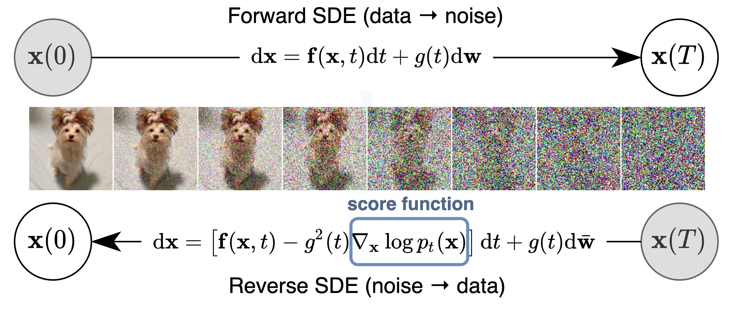
Perturbing data with an SDE
In this case, the noise perturbation procedure is solution of an hand designed SDE of the following form.
\[\boxed{ d\mathbf{x} = \mathbf{f}(\mathbf{x}, t) \, dt + g(t) \, d\mathbf{w}}\]As introduced by Song & Ermon (2021), there are numerous ways to add noise perturbations, and the choice of SDEs is not unique. For example, the following SDE:
\[d\mathbf{x} = e^t \, d\mathbf{w}\]perturbs data with a Gaussian noise of mean zero and exponentially growing variance, which is analogous to perturbing data with
\[\mathcal{N}(0, \sigma_1^2 \mathbf{I}), \, \mathcal{N}(0, \sigma_2^2 \mathbf{I}), \, \cdots, \, \mathcal{N}(0, \sigma_L^2 \mathbf{I})\]when $\sigma_1 < \sigma_2 < \cdots < \sigma_L$ is a geometric progression. Therefore, the SDE should be viewed as part of the model, much like ${\sigma_1, \sigma_2, \cdots, \sigma_L}$.
Reverse SDE for Sampling
Importantly, any SDE has a corresponding reverse SDE (Anderson (1982)), whose closed form is given by:
\[\boxed{d\mathbf{x} = \left[ \mathbf{f}(\mathbf{x}, t) - g^2(t) \nabla_{\mathbf{x}} \log p_t(\mathbf{x}) \right] dt + g(t) \, d\mathbf{w}}\]Here, $dt$ represents a negative infinitesimal time step, since the SDE needs to be solved backwards in time (from $t = T$ to $t = 0$). In order to compute the reverse SDE, we need to estimate $\nabla_{\mathbf{x}} \log p_t(\mathbf{x})$, which is exactly the score function of $p_t(\mathbf{x})$.
Once our score-based model $s_\theta(\mathbf{x}, t)$ is trained to optimality, we can plug it into the expression of the reverse SDE in to obtain an estimated reverse SDE:
\[d\mathbf{x} = \left[ \mathbf{f}(\mathbf{x}, t) - g^2(t) s_\theta(\mathbf{x}, t) \right] dt + g(t) \, d\mathbf{w}.\]We can start with $\mathbf{x}(T) \sim \pi$ where $\pi$ is a well-chosen prior and solve the reverse SDE to obtain a sample $\mathbf{x}$.
Continuous weighted sum of DSM objectives
Solving the reverse SDE requires us to know the terminal distribution $p_T(\mathbf{x})$, and the score function $\nabla_{\mathbf{x}} \log p_t(\mathbf{x})$.
In order to estimate $\nabla_{\mathbf{x}} \log p_t(\mathbf{x})$, we train a Time-Dependent Score-Based Model $s_\theta(\mathbf{x}, t)$, such that
\[\boxed{s_\theta(\mathbf{x}, t) \approx \nabla_{\mathbf{x}} \log p_t(\mathbf{x})}\]This is analogous to the noise-conditional score-based model $s_\theta(\mathbf{x}, i)$ used for finite noise scales, trained such that
\[s_\theta(\mathbf{x}, i) \approx \nabla_{\mathbf{x}} \log q_{\sigma_i}(\mathbf{x}).\]Our training objective for $s_\theta(\mathbf{x}, t)$ is a continuous weighted sum of denoising score matching objectives, given by:
\[\boxed{L(\theta; (\sigma_t)_{t \in \mathbb{R}_{+}}) = \mathbb{E}_{t \sim \mathcal{U}(0, T)} \left[ \lambda(t) \, \mathbb{E}_{\mathbf{x} \sim p} \, \mathbb{E}_{\mathbf{x}_t \sim p_{0t}(\mathbf{x}_t \mid \mathbf{x})} \left[ \left\| s_\theta(\mathbf{x}_t, t) - \nabla_{\mathbf{x}_t} \log p_{0t}(\mathbf{x}_t \mid \mathbf{x}) \right\|^2 \right] \right]}\]where $\mathcal{U}(0, T)$ denotes a uniform distribution over the time interval $[0, T]$, and $\lambda : \mathbb{R} \to \mathbb{R}_{+}$ is a positive weighting function.
Such as before, we will use:
\[\lambda(t) \propto {\mathbb{E}_{(\mathbf{x}_t, \mathbf{x}) \sim p_t(\mathbf{x}_t, \mathbf{x})} \left[ \left\| \nabla_{\mathbf{x}_t} \log p(\mathbf{x}_t \mid \mathbf{x}) \right\|^2 \right]}^{-1}\]to balance the magnitude of different score matching losses across time.
Time-Dependent Score-Based Model
Similar to likelihood-based generative models and GANs, the design of model architectures plays an important role in generating high-quality samples. Since the output of the noise conditional score network $s_\theta(\mathbf{x}, i)$ has the same shape as the input image $\mathbf{x}$, we can draw inspiration from successful model architectures for dense prediction of images (e.g., semantic segmentation).
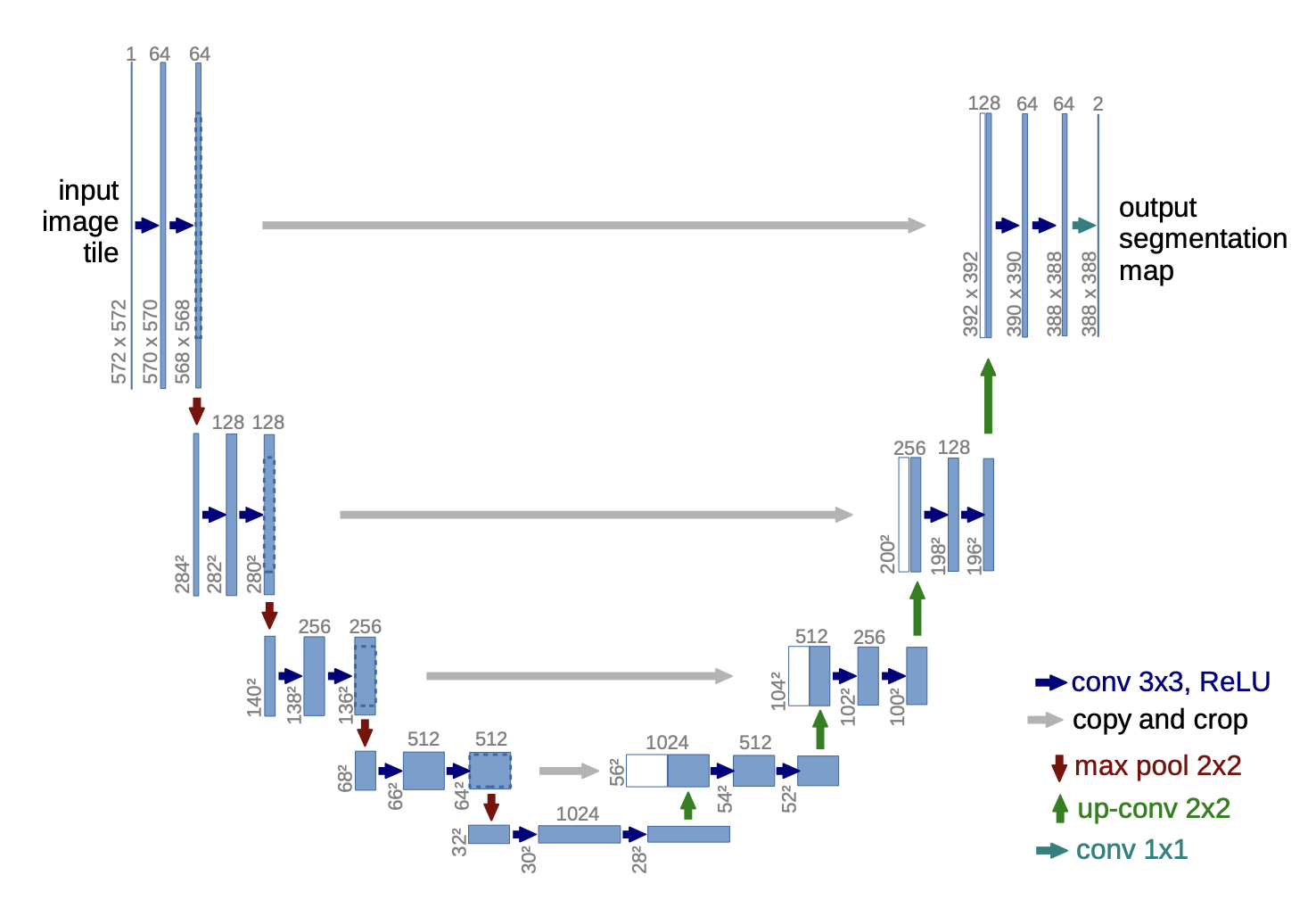
U-net architecture
Typically, we can use the architecture design of U-Net (2015) which have been proved very successful in semantic segmentation. Our goal is then to learn a score function $\nabla_x \log p_t(x)$ that depends on both the noisy input $x_t$ and the time step $t$, using a U-net.
Spectral bias
However, neural networks, particularly MLPs and CNNs (like U-Net (2015)), are not naturally designed to process continuous inputs such as $t$. A naive approach, like feeding raw $t$ values or low-degree polynomial embeddings, often leads to poor generalization—especially when the model needs to represent functions that vary rapidly with time. More precisely, they tend to bias toward learning low-frequency functions (i.e., smooth, slowly varying functions)—a phenomenon known as the spectral bias.
For example, let’s say we have a picture and we want to predict RGB color values for each pixel based on its coordinates using a neural network. Rahaman et al. (2019) observed that enriching input data with high-frequency components facilitates model training. Regular MLPs struggle with learning such functions, which is clearly visible in the blurry image below. However, when we use Gaussian Fourier features proposed by Tancik et al. (2020), we can see that the learned image is much sharper. Enriching input feature space geometry allowed the model to learn high-frequency components much faster:
Time Embedding via Gaussian Fourier Features
Let $t \in \mathbb{R}$ be a continuous scalar (the time step), and let $\mathbf{W} \in \mathbb{R}^{D/2}$ be a vector of random frequencies sampled from a normal distribution:
\[\mathbf{W}_i \sim \mathcal{N}(0, \sigma^2)\]We define the embedding:
\[\gamma(t) = \left[\sin(2\pi t \cdot \mathbf{W}),\ \cos(2\pi t \cdot \mathbf{W})\right] \in \mathbb{R}^{D}\]This transforms the 1D input $t$ into a $D$-dimensional representation capturing multiple frequency bands. The sinusoidal structure ensures that nearby values of $t$ can be linearly combined to reconstruct complex functions, while the random frequencies help to decorrelate different components. In practice, this embedding behaves similarly to a positional encoding (as in Transformers (2017)), but generalized to continuous domains using random projections.
References
-
Reverse-time diffusion equation models — Anderson, B. D. O. (1982).
-
Density Estimation Using Real NVP — Dinh, L., Sohl-Dickstein, J., & Bengio, S. (2016).
-
Generative Adversarial Nets — Goodfellow, I. et al. (2014).
-
Estimation of Non-Normalized Statistical Models by Score Matching — Hyvärinen, A. (2005).
-
Auto-Encoding Variational Bayes — Kingma, D. P., & Welling, M. (2013).
-
On the Spectral Bias of Neural Networks — Rahaman, N. et al. (2019).
-
U-Net: Convolutional Networks for Biomedical Image Segmentation — Ronneberger, O., Fischer, P., & Brox, T. (2015).
-
Generative Modeling by Estimating Gradients of the Data Distribution — Song, Y., & Ermon, S. (2020).
-
Score-Based Generative Modeling through Stochastic Differential Equations — Song, Y., Sohl-Dickstein, J., Kingma, D. P., Kumar, A., Ermon, S., & Poole, B. (2021).
-
Fourier Features Let Networks Learn High Frequency Functions in Low Dimensional Domains — Tancik, M. et al. (2020).
-
Attention Is All You Need — Vaswani, A. et al. (2017).
-
A Connection Between Score Matching and Denoising Autoencoders — Vincent, P. (2010).